Troubleshooting
Creating Top 10 List Without Pivot Table

Creating a top 10 list without pivot table is actually pretty easy. But creating a decent one needs some effort. I am going to create a monthly top 10 customers list that can be filtered by month. Here is the step by step introductions for how to do it:
This is our base data that contains monthly purchases. For our top 10 list, we need a customer based data.
Here is our customer based data. Purchases by month are calculated with a Sumifs Function in the last column. Not all customers made purchases each month, so don’t worry if you see zeros in this column.
Now let’s setup our top 10 list. I setup my workbook as shown below. Columns P to S will be hidden in final form.
Here you can see that I fetched top 10 purchases by using Large Function. I also went to some extra lengths to provide a nicer month filter.
Now we need to fetch customer names and surnames for each monthly purchase. This part is a little tricky because there might be more than one customers who made same amount of purchases. If we use regular lookup methods, we might end up fetching first name in the list for that purchase for each occurrence.
I will use the same method I used for Finding 2nd Matching value with Vlookup.
I will add a helper column to make purchase occurrences unique, so I can fetch right name each time. Here is my monthly purchases data with helper column added. As you can see, new column has purchase value with an occurrence counter attached to it.
I need to do same thing for my top 10 list too. Rest is typing a lookup formula into the name field. I used an Index+Match Formula since my helper column is the rightmost column. You can do this with Vlookup Function too. But your helper column should be located left of name column in that case. I’d really recommend learning Index+Match Formula though. It is an absolute life saver. Here is how it looks at this point:
Now that getting names for purchases is done, we need to fetch matching surnames. The reason and process is absolutely same with name field. Just repeat same helper column creations and your list is finished.

Slicers is a very useful but underutilized tool in Excel. You can dynamically filter your pivot tables and pivot charts with animated buttons, aka slicers. For more information on slicers, you can check this short article.
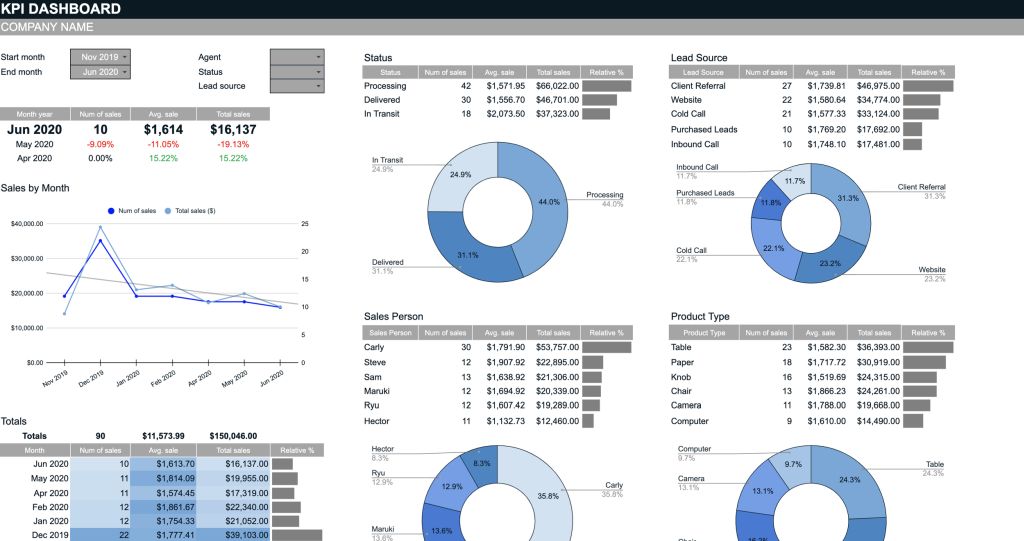
Now let’s see how to build an Interactive Excel KPI Dashboard using pivot table tools:
I prepared a summary data for 4 departments; welding, cutting, assembly and packing. KPI’s for these 4 departments are selected as efficiency, productivity and scrap rate. Data set includes values for 12 months (4x3x12=144 rows). Here is how data set looks:
Select all the data and insert a pivot table. Arrange fields as shown below (Don’t look for Rest field at this point. We are going to add it in next step):
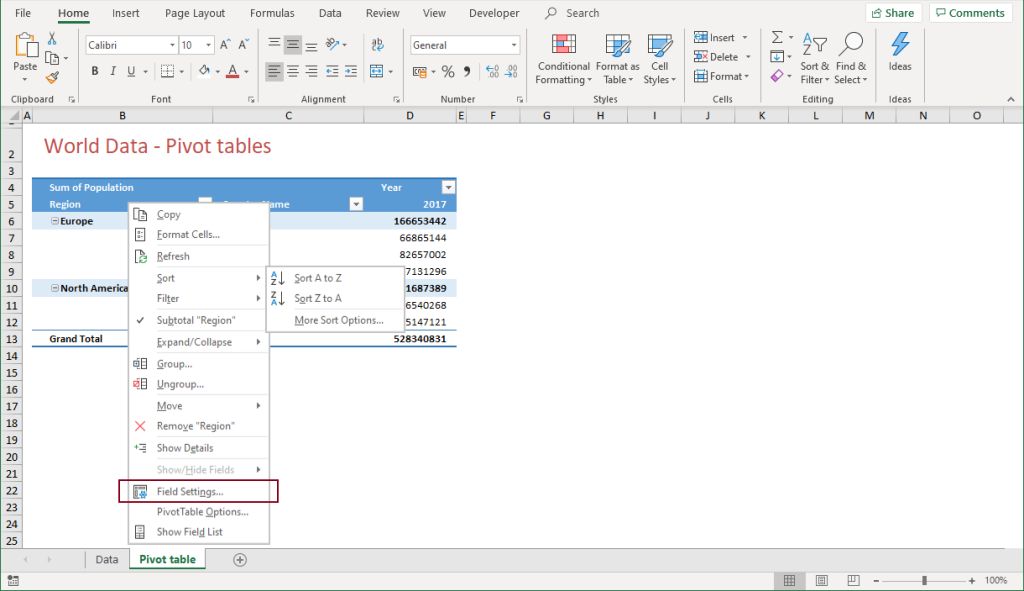
Click on the pivot table to activate it and add a calculated field from the menu shown below:
Set calculated field parameters as shown below and we will have an additional field in our pivot table to use for our charting needs:
Set KPI filter as “Productivity” and make 2 copies of the pivot table (by copy and paste). Set KPI filter for those tables as “Efficiency” and “Scrap Rate”. Here is how it is supposed to look:
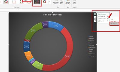
Insert a donut chart for each of these pivot tables. Cut them and paste them to another sheet. Format your charts to look like this:
To do this, right-click on any gray button on the chart and select “Hide All Field Buttons on the Chart”. Delete chart title and legend. Then click on the donut and set shape outline to “No Fill”. Set shape color separately by clicking on them and selecting color.
Now make another copy of the first chart and arrange fields as shown below:
When finished, make 2 copies of this pivot chart too:
Now merge 3 cells and type “=B5” (without bracelets). B5 is the cell that contains result value of first pivot table (you can see from previous picture). Make sure to disable gridlines here. Then select your merged cell and copy it. Then paste it, as linked picture, to the sheet that has your donut charts. And drag it over related chart.
We are finished our donut charts at this point. It is time for our column charts. We need a 3 column data table for each of our column charts. Here is how I do it:
Place a 3 column grid just under the second set of pivot tables. First row will contain column titles. First column will contain month names. Remaining 2 columns will be filled by formulas. Here are the formulas:
Result Column Formula:
=SUMIFS(Sheet1!$E:$E;Sheet1!$A:$A;Sheet2!$A$14;Sheet1!$B:$B;Sheet2!$B$11;Sheet1!$D:$D;Sheet2!$A20)
This formula fetches result values based on department and KPI values selected on the pivot table above and month name in first column. You can see how to use this function from here SUMIFS FUNCTION.
Selection Column Formula:
=IF(A20=$A$15;B20;NA())
This formula checks selected month on the pivot table above and shows result value from 2nd column if month matches. If it doesn’t match, it shows #N/A.
Here are the tables I prepared:
Now select first table and insert a column chart. For formatting:
- Double-click on the orange column and set is as secondary axis.
- Set Series Overlap and Gap Width to 100%
- Delete both axes, chart title, legend and grid lines.
- Change column colors and set Shape Outline for the chart as “No Fill”
Here is how your chart should look like after all these make-up:
Do the same for other tables (other KPI’s), you can also copy chart formatting to do this faster. Then place these chart next to your donut charts:
Now comes the interactivity part. Click on your first donut chart and insert a slicer from INSERT ribbon. Select Month Name as field. Make sure settings are made as shown below:
You should check whether your slicer works correctly, by clicking on its buttons. If it doesn’t change charts, it is most likely because of report connections. You can correct this issue from there. Insert slicer for other KPI’s (chart pairs) too.
Now customize you slicers as a 3×4 button grid with button height and width as 1,2cmx1,2cm. Change colors to match with your charts. You can see how to do this from Customize Slicers. Here is how it should look like:
Add a final slicer for departments. You can do this by clicking on any of the charts and inserting a slicer. This slicer must be connected to all pivot tables.
Place it on top of your charts, add KPI texts over slicers and our dashboard is done.
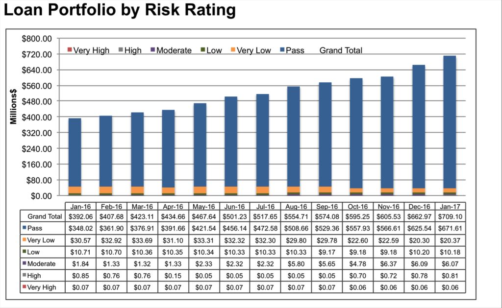
When one value on your chart is much higher than the rest, lower values on your chart might become unreadable. In this tutorial, you will learn a net way to deal with this kind of situations.
As you see, smaller values are almost indistinguishable due to chart scaling to show all values together.
We want to show all values together in the same chart too, but we also want them to be clearly understandable. Therefore, we have to crop this towering value to make it scalable.
To achieve our goal, we need to make a couple of little adjustments to our data set:
- Add 3 columns next to our original data. First column values will be the same for each series except the one with the high value. Give it a value just a little higher than the second higher value.
- Second and third columns will have “=NA()” as values for all series except the one with the high value. For second column, give it a value that will create a gap. And for third column, give it a little bigger value but not bigger than the first column value.
- Insert a stacked column chart by selecting whole data, than uncheck “Production” series from your source list.
- Your chart is supposed to look like the one in the picture below.
- Now we are going to format this chart to mate it look like the one below:
Here are the formatting I made on my chart:
- Add a chart title.
- Change color of the third column value on the chart to match the color of other series.
- Change fill of the second column value on the chart as pattern fill. Select vertical lines as pattern.
- Add labels for the first column values and move them above the bars.
- Add a label to the top of he longest series as a test box and write the original high value in it.
This is an easy way to create a chart with high and low values which shows all values together without compromising readability.

Summary: The blog summarizes the methods to repair MS Excel workbook and explains various benefits that each procedure offers. It also describes a third-party Excel Repair tool for a successful recovery of data from 0 KB Excel file error message (when excel file size become 0 kb).
While attempting to access Excel workbook, if you encounter an 0 KB file error message (excel file size become 0 kb), the chances are that your file is corrupt or the version of the file you use is not compatible with the Excel edition. The error message reads as follows:
“Excel cannot open the file ‘filename.xlsx’ because the file format for the file extension is not valid. Verify that the file has not been corrupted and that the file extension matches the format of the file.”
Excel provides a few troubleshooting procedures that users may execute to repair the workbook. These workaround methods are easy to execute; however, doing so may also lead to permanent loss of data unless you are technically adept. Before following any of the recovery methods, it is recommended that you create a backup of your Excel file.
Method #1: Excel File Recovery Mode
MS Excel automatically starts File Recovery mode upon opening, when any corruption is detected in the Workbook. You can also follow the manual procedure to open the File Recovery mode if it doesn’t start automatically.
Follow the steps below to manually start the File Recovery mode:
- Click on the File tab and then click on Open
- Click the folder where the corrupt file exists
- In the Open dialog box that appears, select the damaged workbook
- Click on the arrow button available next to Open button and select Open and Repair
- To repair maximum data from the corrupt workbook, click on Repair
If Repair fails to recover the data, select Extract Data for extracting formulas and values from the Excel workbook.
Method #2: If Workbook Opens in Excel
Revert Workbook to the Last Saved Version
In case the Workbook turns corrupt while working on it, you may not be able to save the changes. In such a scenario, you can revert the Workbook to last saved or the previous version. To do so:
- Click on File and then click on Open
- Double-click on the Workbook name
- Next, click Yes to reopen
Note: You may lose the changes made recently to the Workbook as it will open without any changes that have turned Workbook corrupt.
Method #3: When Workbook Cannot Open in Excel
Set Calculation Option to Manual
If you are not able to open the Workbook in Excel, then attempt to change the calculation setting to manual from automatic as it may open in Excel as it cannot be recalculated thereafter.
- Click on the File tab and then click on New
- Click on the Blank workbook available under New
- Next, click on File and then select Options
- Under Calculation Options in the Formulas category, select Manual and then OK
- Next, click on File and then click on Open
- Search and find the corrupt Workbook and then double-click to open
Method #4: Use External References
You may try using external references to link to the damaged workbook; however, it will help retrieve only data from the Workbook. Other contents such as calculated values and formulas can be dropped for retrieval. The entire procedure to use external references to links to the corrupt workbook is considerably complicated and hence requires someone with a good technical know-how.
Method #5: Save from Backup
If a backup is available, you can access your lost data if the workbook turns corrupt. To automatically restore the backup, follow the steps below:
- Click on File and then click on Save As
- Click on Computer and select the Browse button
- In the then appeared Save As dialog box, select the arrow sign available next to the Tools button. Then select General Options.
- In the General Settings dialog box that appears, check the box associated with Always create backup box
Method #6: Third-Party Recovery Assistant
You may also opt for third-party applications to resolve your Excel file 0KB issue. Not only would they resolve all types of XLS and XSLX issues, but their easy to use interface allows for a seamless recovery. Stellar Phoenix Excel Repair is one such software. With it, you can simply repair the file from any type of corruption, from smaller to a higher level. All the contents of the Excel workbook such as charts, rules, properties, texts, engineering formulas, etc. can be restored back on the machine effortlessly.
The recovery procedure is simple to execute. This Excel Repair software can be run on all the versions of Windows OS. It supports all versions of Excel, from the oldest to the most recent editions.
The tool is simple to execute and doesn’t require you to have any specific technical expertise. It easily resolves the 0KB Excel file issue and retrieves the corrupt data. All recovered data is saved in a new file at the desired location while the older files remain intact.
The Way Forward
MS Excel is an indispensable part of a professional day-to-day life. With it, managing and analyzing data to support your decision-making and other business outcomes becomes easy. Therefore, its importance cannot be discounted. It is always recommended to take preventive measures to safeguard your Excel files from turning corrupt; however, if it becomes corrupt, then employing a secure and reliable tool is recommended.
-
 Education11 months ago
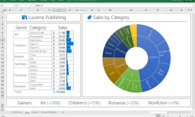
Excel Sunburst Chart
-
 Education1 year ago
Fix Microsoft Excel Error – PivotTable Field Name Is Not Valid
-

 Excel for Business8 months ago
Interactive Excel KPI Dashboard
-

 Education12 months ago
Positive Negative Bar Chart
-

 Education1 year ago
Excel Gantt Chart (Conditional Formatting)
-
 Excel for Business1 year ago
Mastering Chart Elements in Excel to Unlock Better Data Visualization
-

 Education12 months ago
Word Cloud Generators: The Modern Tool for Simplifying Data Visualization
-
 Education1 year ago
Streamlining Election Vote Counting with an Excel Election Template